Normal Distribution

Definition

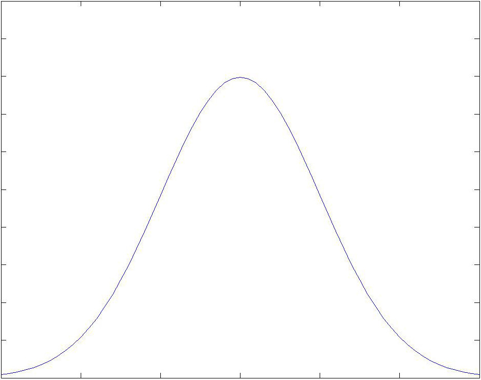
Let $X$ be a continuous random variable. Then $X$ takes on a normal distribution with parameters $\mu$ (the mean) and $\sigma$(the standard deviation), denoted $X \sim \mathrm{N}(\mu, \sigma^2)$, if its probability density function is \[f(x) = \dfrac{1}{\sigma \sqrt{2 \pi}} \mathrm{exp}\left(-\frac{1}{2} \left( \frac{(x-\mu)}{ \sigma} \right)^2 \right)\text{.}\]

The normal distribution is a very common distribution and it's very useful to statisticians, in particular because of the central limit theorem which states that the mean of many independent random variables, $X_1, X_2, \ldots , X_n$ from the same distribution is approximately normally distributed. We will look at a special case of the normal distribution called the standard normal distribution which is a little easier to work with.

Standard Normal Distribution

Definition

Let $X$ be a continuous random variable. Then $X$ takes on a standard normal distribution if its probability density function is \[f(x) = \dfrac{1}{\sqrt{2 \pi} }\mathrm{exp}\left(-\frac{1}{2}x^2\right)\text{.}\] In other words, the standard normal distribution is the normal distribution with mean $\mu=0$ and standard deviation $\sigma = 1$. So now we have a pdf which is a little easier to work with. But what if the random variable $X$ doesn't have mean $\mu = 0$ or standard deviation $\sigma = 1$?

Fortunately, we can take any continuous random variable $X$ which is normally distributed and convert it to a continuous random variable $Z$ which has the standard normal distribution.

Converting Normal to Standard Normal

To convert $X$ to $Z$ use the formula \[Z = \dfrac{X - \mu}{\sigma}.\]

Let's think about what this does. We have a normally distributed random variable $X$ with mean $\mu$ and standard deviation $\sigma$. By taking away $\mu$ we shift the graph to either the left or the right until the mean is $0$. By dividing by $\sigma$ we change how far across the data is spread until the standard deviation is $1$ (recall the standard deviation is a measure of how far the data is spread from the mean).

We can obtain that \[\mathrm{P}[X \leq x] = \mathrm{P}\left[ \dfrac{X- \mu}{\sigma} \leq \dfrac{x-\mu}{\sigma} \right] = \mathrm{P}\left[ Z \leq \dfrac{x-\mu}{\sigma} \right] = \Phi \left(\dfrac{x-\mu}{\sigma} \right) = \Phi (z)\] where $\Phi$ is the cumulative distribution function and $z = \frac{x-\mu}{\sigma}$. To see why, click here.

This means that the probability that $X$ is less than $x$ is the area under the graph of the standard normal distribution between $-\infty$ and the corresponding $z$ value. Rather than having to calculate this area, a table is provided for each positive $z$ value. Because the normal distribution is symmetric, this can be used to calculate the probability when negative $z$ values are obtained as well.

The definition of the standard normal distribution ensures that the area under the standard normal curve is $1$.

Normal Approximation to the Binomial Distribution

In some circumstances, calculating a probability with the binomial distribution can take a long time. For example, given a random variable $X$, if $X \sim \mathrm{Bin}(4000, 0.8)$ and we want $\mathrm{P}[X>3500]$ we would have to calculate \[\mathrm{P}[X=3501] + \mathrm{P}[X=3502] + \ldots + \mathrm{P}[X=4000]\text{.}\] It can be more efficient to use the normal distribution with the same mean and standard deviation to approximate the binomial distribution.

Let $Y$ be this approximation. From the binomial distribution we have $\mu = np = 3200$ and $\sigma^2 = np(1-p) = 640$. So $Y\sim \mathrm{N}(3200, 640)$. The approximation we use is \[\mathrm{P}[X=x] \approx \mathrm{P}\left[x-\frac{1}{2} \leq Y \leq x+\frac{1}{2}\right]\text{.}\] For example \begin{align}\mathrm{P}&[X=3750] \approx \mathrm{P}[3749.5 \leq Y \leq 3750.5]\text{,}\\ \mathrm{P}&[2500\leq X \leq 2600] \approx \mathrm{P}[2499.5 \leq Y \leq 2600.5]\text{,}\\ \mathrm{P}&[X>3500] \approx \mathrm{P}[3499.5 \leq Y \leq 4000.5]\text{.} \end{align}

Conditions

To approximate the binomial distribution with the normal distribution, the following two conditions must hold:

• $np>5$
• $n(1-p)>5$.

Reading the Tables

Once we obtain a $z$ value, we can use the cumulative probability tables of the Normal Distribution to find out the probability that $Z$ is less than (or “less than or equal to”, we obtain the same value either way because we have a continuous distribution) the $z$ value we have obtained.

Usually we will get a $z$ value to 2 decimal places. We need to split this up. For example \begin{align} 2.22 &= 2.2+0.02 \\ 1.75 &= 1.7+ 0.05 \\ 1 &= 1.0+0.00 \end{align}

Once we have split it up, we take the first part and look down the left hand column until we get to this number and highlight the corresponding row. The second part will always be between $0.00$ and $0.09$ so we go along the top row until the number is found. Now we follow this column down until we reach the row highlighted earlier. The number where the highlighted row and column meet is the probability that $Z$ is less than our $z$ value.

Worked Example

Given that $z=0.76$:

a) What is the probability that $Z$ is less than $z$?

b) What is the probability that $Z$ is greater than $z$?

c) what is the probability that $Z$ is less than $-z$?

Solution

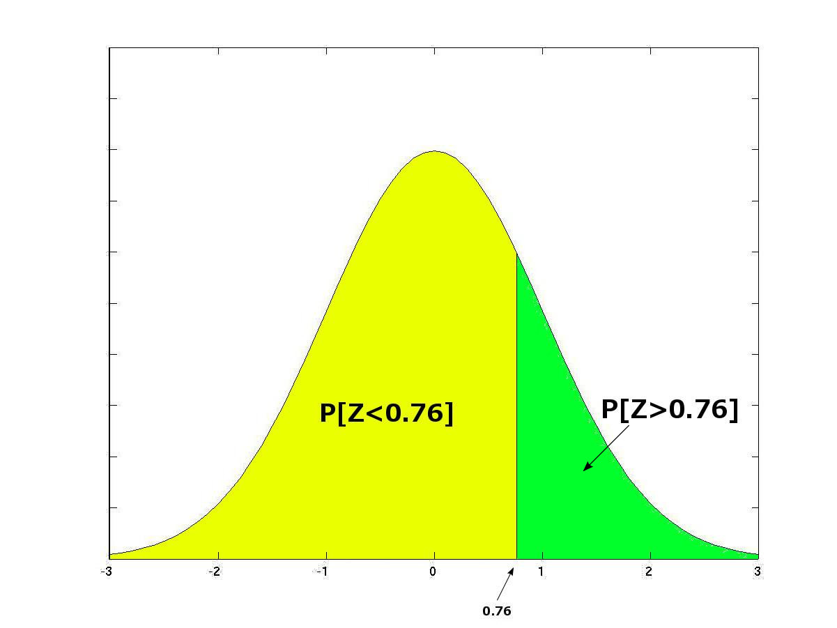
a) Split $z=0.76$ into $z=0.7 + 0.06$. Look down the first column for $0.7$ and highlight the row it is on. Now look along the first row for $0.06$ and look down that column until we reach the highlighted row. The point where these two meet is the probability, giving in this case $0.7764$.

b) The probability that $Z$ is greater than $0.76$ is the same as the probability that $Z$ is not less than $0.76$ (recall for the normal distribution, as for all continuous distributions, $\mathrm{P}[X

\begin{align} \mathrm{P}[Z>0.76] &= 1 - \mathrm{P}[Z<0.76] \\ &= 1-0.7764 \\ &= 0.2236 \end{align}

c) This time we need the probability that $Z$ is less than $-0.76$. The tricky bit here is the $-$. The standard normal distribution is symmetric about $0$ so the area between $-\infty$ and $-0.76$ will be the same as the area between $0.76$ and $\infty$.

So \begin{align} \mathrm{P}[Z<-0.76] &= \mathrm{P}[Z>0.76] \\ &= 1 - \mathrm{P}[Z<0.76] \\ &= 1-0.7764 \\ &= 0.2236 \end{align}

Worked Examples 1

Worked Example

Video Examples

Example 1

In this video, Dr Lee Fawcett solves a problem involving finding the probability that a measurement from a normal distribution is less than a certain amount.

Example 2

In this video, Dr Lee Fawcett explains how to find probabilities from a general normal distribution using a table of values from the standard normal distribution.

Workbooks

These workbooks produced by HELM are good revision aids, containing key points for revision and many worked examples.

• The normal distribution
• The normal approximation to the binomial distribution

External Resources

• Slides on the Normal Distribution at MIT

• Normal distribution at Science Online Classes

See Also

Hypothesis Testing with the Normal Distribution