Continuous Probability Distributions (Animal Science)

Continuous Probability Distributions

When we are dealing with continuous probability distributions, we always look at the probability that a random variable lies within a particular range of values. For example, we might want to know the probability that the weight of a ram of a particular breed is in the range $90-100$kg or the probability that it is greater than $120$kg.

For a continuous probability distribution, a curve called a probability density function or pdf contains the information about these probabilities. The probability that a continuous random variable lies in a given range is equal to the area under the probability density function curve in that range. The total area under the curve for any pdf is always equal to $1$, this is because the value of a random variable has to lie somewhere in the sample space. In other words, the probability that the value of a random variable is equal to 'something' is $1$.

The Normal Distribution

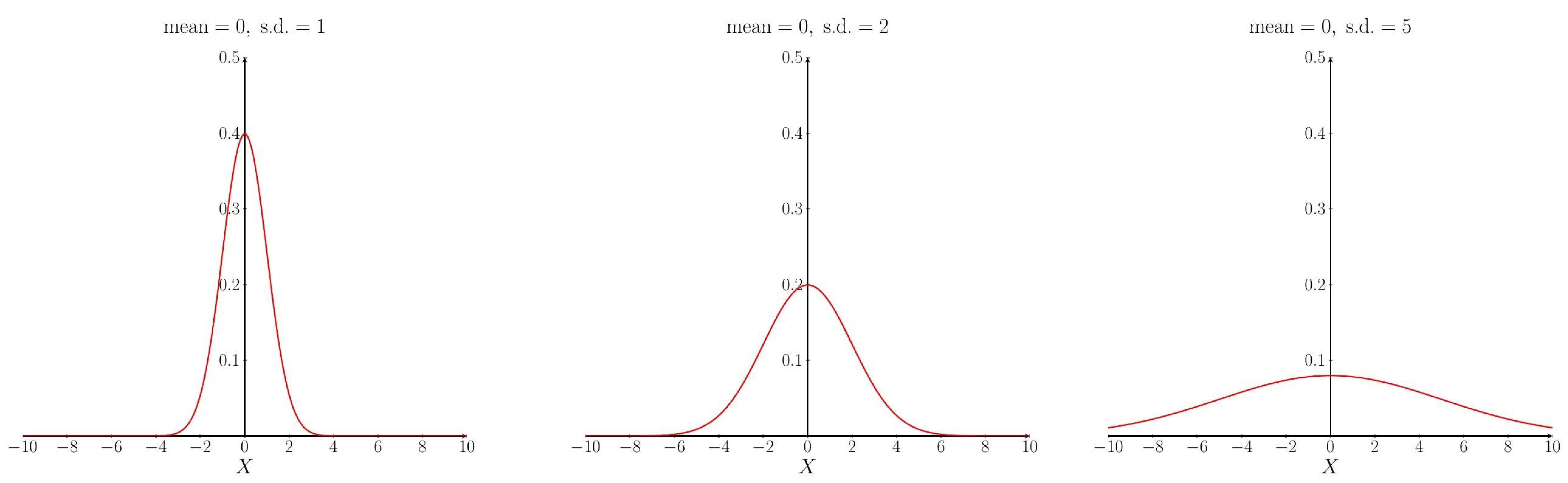
The Normal or Gaussian distribution is possibly the best-known and most-used continuous probability distribution. The Normal distribution is a good approximation to many statistics of interest in populations such as height and weight. The probability density function (pdf) for a Normal distribution has a bell-shaped profile.

Although the plot only shows the curve in the range $X$ goes from $-5$ to $+5$, the curve goes all the way out to minus infinity and plus infinity. There is a formula for the pdf curve that contains two parameters, the mean and the standard deviation (s.d.). Changing these parameters changes the pdf curve. Changing the mean changes where the location of the curve on the $X$ axis, increasing the mean moves the curve to the right, decreasing the mean moves the curve to the left. Changing the standard deviation changes how spread out the curve is.

Working Out Probabilities

Suppose we have a random variable $X$ which has a Normal distribution with mean $0$ and standard deviation (s.d.) $1$. If we want to know the probability that $X$ lies in the range $0$ to $1$ then this is equal to the area of the shaded region on the graph shown below.

It is actually a bit tricky to calculate areas like this but luckily there are tables available for the Normal distribution which we can use to look up the probabilities, there are also computer packages such as R and Minitab which can tell us the probabilities. If you would like to read a little more about reading probability tables for the Normal distribution you can do so here (a little reading about the notation is required before looking at the section on reading the tables). From the tables, we find that the shaded area above is equal to $0.3413$.

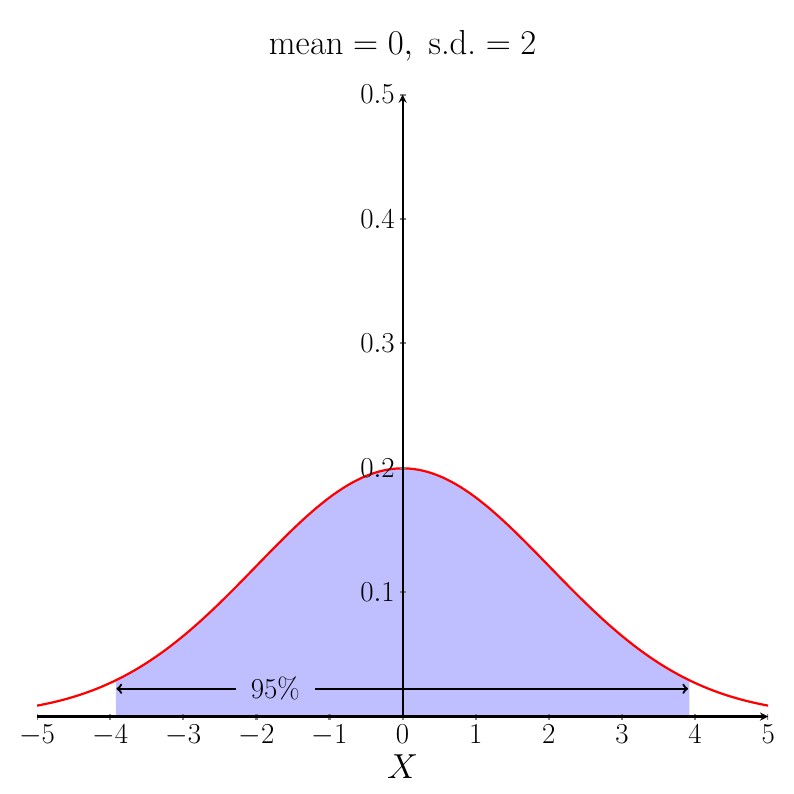
Whatever the mean and s.d. are equal to, $95\%$ of the area under the Normal distribution pdf curve lies in the range [mean $- 1.96 \times $ s.d.] to [mean $+ 1.96 \times$ s.d.]. This fact is often used in the calculation of a reference range. A good way to remember this is that $95\%$ of the area under the curve lies within roughly $2$ standard deviations of the mean. The figure below shows the case when the mean is $0$ and the s.d. is $2$.

Other Continuous Probability Distributions

There are lots of continuous probability distributions apart from the Normal distribution. In particular, you will probably meet the Student's t-distribution or t distribution and the Chi-squared ($\chi^2$) distribution. The t-distribution is used when testing a hypothesis about a mean or a difference between two means and the Chi-squared distribution is used when analysing categorical data.