Linear Equations (Business)
Linear Equations
Linear equations are equations of straight lines and are of the form $y = ax + b $ or $ax + by = c $ (where a $a, b,$ and $c$ are constants i.e. they do not change when $x$ or $y$ change). These equations are called linear because neither of the variables $x$ or $y$ is raised to a power other than one or zero and they have constant coefficients (the letters in front of the variables are constants). Without these properties the equations would not be nonlinear. See below for more examples.
The gradient (slope) of a straight line is calculated as the change in two $y$ values divided by the change in the two corresponding $x$ values and is denoted:
$\dfrac{\triangle y}{\triangle x} = \dfrac{y_2 - y_1}{x_2 - x_1}$ where $y_2 > y_1 \text{ and } x_2 > x_1$ (see below diagram for identifying these points).
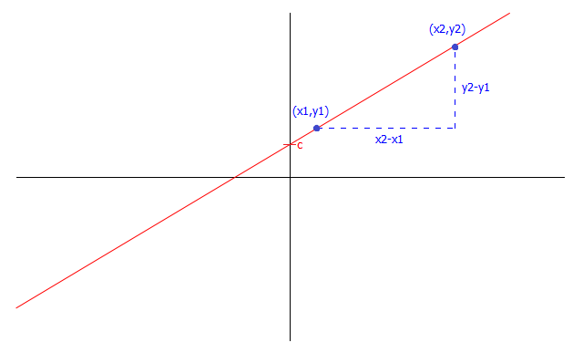
' Note:' Gradients can be positive (where an increase in the value of $x$ results in a increase in the value of $y$), negative (where an increase in the value of $x$ results in a decrease in the value of $y$) or you can have a zero gradient (where changes in $x$ result in no change in the $y$ value i.e. a horizontal line).
Worked Example 1
Worked Example - Linear or Nonlinear?
Decide whether the following equations are linear or nonlinear: a) $ \text{}y = 4x^2 + 4 + 5x$
b) $\text{} 9990 = 99y - 578x $
c) $\text{}4567 = 23xy$
Solution
a) This is a nonlinear equation as $x$ is squared (raised to the power of 2).
b) This is a linear equation as it is in the correct form: neither $x \text { nor } y$ is raised to a power other than one or zero and their coefficients are constants.
c) This is a nonlinear equation as $x \text{ and } y$ are multiplied together so the coefficients of $x $ and $y$ are not constant.
If you are unsure on whether an equation is linear or not try plotting it. (To do this you could use R, wolframalpha or excel etc.)
Sketching Linear Equations
We can understand equations more by sketching them. Given an equation of the form $y = ax + b$, for each value of $x$ you substitute this value of $x$ into the equation (i.e. multiply it by $a$ and add $b$) to obtain the corresponding $y$ value. On the graph you put a mark at each of the points where your chosen values of $x$ and the corresponding values of $y$ intersect (i.e. the coordinate $(x,y)$ for each $x$ and corresponding $y$). Once you have a few points, sketch a line through them.
Worked Example 2
Worked Example
Sketch the graph of $y = 2x - 3$ and calculate the gradient.
Solution
To sketch $y = 2x - 3 $ you substitute a few values for $x$ in and obtain the $y$ coordinates, add these to your graph and sketch a line through the points.
For instance some pairs of values are :
$(0, - 3)$, when $x = 0,\;\;y = (2\times 0) - 3 = - 3 $ and
$(4, 5)$, when $x = 4, \;\;y = (2\times 4) - 3 = 5$ .
By repeating this for other values of $x$ you can obtain the straight line shown on the graph below:

|center
To calculate the gradient of the above straight line use the formula $\dfrac{\triangle y}{\triangle x}$. Since the gradient of a straight line is constant throughout the straight line we can calculate the gradient between any two points on the line.
The gradient between the above points $(0, - 3)$ and $(4,5)$ is:
$\dfrac{5 - (- 3)}{4 - 0} = \dfrac{8}{4} = 2$ meaning the straight line has a positive gradient i.e. an increase in $x$ corresponds to an increase in $y$.
' Note:' if you are given an equation of a line in the form $y = ax + b$ then $a$ is the gradient and $b$ is where the line intercepts (crosses over) the $y$-axis.
Using Linear Equations for Modelling
The relationships given by linear equations and can be used to create models for business situations such as supply and demand equations or production costs and budget constraints.
You do not only work with linear equations in the variables $x$ and $y$, other variables are commonly used. For instance, when making models of demand and supply $Q$ is often used for quantity demanded and $P$ for price.
For example, the equation $Q =3999 - 3P$ might be appropriate as it implies that demand decreases when the price increases.
This equation can be rearranged to make $P$ the subject as follows: $P = 1333 - \dfrac{Q}{3}$.
So, if given the quantity demanded, you can calculate the corresponding price by substituting the value of $Q$ into this equation.
Test Yourself
Try our Numbas test on linear programming
See Also
For developing the techniques seen in this section further see rates of change.