Linear Programming (Business)
Linear Programming
In business and elsewhere we are constrained by the limited availability of resources such as time, people, money, supply of materials etc..
We must work with these constraints in a way that enables us to still meet our objectives as best we can. These objectives could include maximising profits, minimising stock, minimising costs or a combination of such objectives.
In this section we briefly explain the technique of linear programming and give some simple examples. The term linear programming is used here as the constraints are given by linear inequalities involving the main resources under your control and your objective can also be expressed in terms of a linear combination of these resources.
An example of a linear inequality
You have at most £$1000$ with which to buy presents for boys and girls at an orphanage. The boys' presents cost £$10$ each and the girls' presents cost £$7$ each. Let $x$ represent the number of boys' presents and $y$ represent the number of girls' presents.
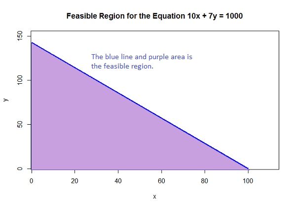
The possible allocations of the presents can be expressed as a linear inequality: \[10x + 7y \le 1000\] which reflects the constraint that you have at most £$1000$ to spend. Any pair of values of $x$ and $y$ which satisfy this equation is called a feasible solution.
The graph below highlights the feasible region for values of $x$ and $y$. This region includes all feasible solutions. Note that this is further constrained by $x$ and $y$ having to be integers (and also that $x \ge 0,\;y \ge 0$). The decision regarding what particular values of $x$ and $y$ from all possible such values (highlighted in the graph) to choose from cannot be made unless we have some other constraints or rules given.

|center
Solving Linear Programming problems graphically
As in all linear programming models, you first create linear inequalities out of the information you have about any constraints.
In the case of profit maximisation or loss minimisation, for example, your objective function will be a linear combination of the production resources you have control over and that you can vary. Your task is to find the values for these production resources which meet the constraints and maximise (in the case of profit) or minimise (in the case of costs) the objective function. In the example below you have to maximise profit.
First sketch the lines of the constraints given by the linear inequalities on a graph, and the common area under these lines is the feasible region of values as this is the region where all inequalities are satisfied.
The next step is to find the point in the feasible region which gives the optimum value for the objective function. This usually occurs at a point on the boundary of the feasible region and can be found by looking at the value of the objective function and where it intersects the boundary and choose the optimum value.
This method is demonstrated in the example below.
Worked Example
Worked Example
A bakery makes two brands of cake, Slimming-watchers and Scrumptious. For a single batch of Slimming-watchers cakes they require 3kg of sugar and 7kg of butter, while for a single batch of Scrumptious cakes they require 11kg of sugar and 13kg of butter. The bakery makes £6.50 profit on a batch of Slimming-watchers cake and £9 profit on a batch of Scrumptious cake. The bakery has access to at most 700kg of sugar and 1150kg of butter per day.

How many batches of Slimming-watchers and Scrumptious cakes should the bakery produce each day to maximise profit? Formulate this as a linear programming problem and solve the problem graphically.
Solution
Let $x$ be the number of batches of Slimming-watchers cakes and $y$ the number of batches of Scrumptious cakes. These are the production resources we have control over.
Objective function Since $x$ batches of Slimming-watchers cakes produces a profit of £$6.5x$ and $y$ batches of Scrumptious cakes produces a profit of £$9y$, the the total profit is given by £$6.5x + 9y$. This is the linear objective we want to maximise.
Constraints The constraints on the ingredients can be written as inequalities as follows:
Sugar: $3x +11y \leq 700$ and
Butter: $7x + 13y \leq 1150$.
And of course $x \ge 0,\; y\ge 0$.
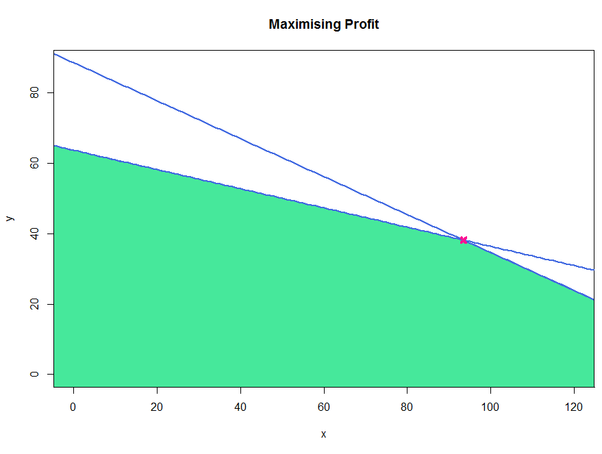
Graph To solve graphically, we sketch the lines $3x+11y = 700$ and $7x + 13y = 1150$ (see graph).
The feasible region is the area that is enclosed by both of these lines and the $x$ and $y$ axis (green area on below graph).
The maximum of $6.5x + 9y $ lies on one of the three corner points of the feasible region.
The intersect is the solution to the pair of equations:
- $3x + 11y = 700$
- $7x +13y =1150$
which you solve using the method shown above to get $x = \dfrac{1775}{19} $ and $y = \dfrac{725}{19}$
The other corner points are $\left( \dfrac{1150}{7}, 0\right)$ and $\left(0, \dfrac{700}{11}\right)$

To find which point maximises profit, we substitute into the equation $6.5x + 9y$. Substituting the three coordinates into this equation we obtain:
- The profit at $\left(\dfrac{1150}{7}, 0\right)$ is $1067.86$
- The profit at $\left(0, \dfrac{700}{11}\right)$ is $572.73 $
- The profit at $\left(\dfrac{1775}{19}, \dfrac{725}{19}\right) $ is $950.66$.
So we obtain the maximum profit at $\left(\dfrac{1150}{7}, 0\right)$. We can conclude the bakery needs to make $164$ (we round down as we must make whole batches) batches of Slimming-watchers cake and zero batches of Scrumptious cake each day to make the most profit.
Test Yourself
Try our Numbas test on linear programming
See Also
For developing the techniques seen in this section see rates of change.