Exponential Distribution (Business)
Exponential Distribution
The Exponential Distribution is another important distribution and is typically used to model times between events or arrivals.The distribution has one parameter, $\lambda$ which is assumed to be the average rate of arrivals or occurrences of an event in a given time interval.
If the random variable $X$ follows an Exponential distribution then we write: $X \text{~}\mathrm{Exp}(\lambda)$.
The probability density function is:
\[f(x)= \begin{cases} \lambda e ^{-\lambda x} & \text{for }x \geq 0, \\ 0 &\text{otherwise}. \end{cases}\]
(Cumulative) probabilities can be calculated using:
\[\mathrm{P}(X \leq x) = \begin{cases} 0 & \text{for }x \lt 0, \\ {1} - e^{-\lambda x} & \text{for } x \geq 0. \end{cases}\]
Expectation and Variance
The expectation and variance of an Exponential random variable are:
\begin{align} \mathrm{E}[X] &= \dfrac{1}{\lambda}\\ \mathrm{Var}(X) &= \dfrac{1}{\lambda^2}\\ \end{align}
Worked Example 1
Worked Example
It is assumed that the average time customers spends on hold when contacting a gas company's call centre is five minutes. The company has a policy that if a customer waits for longer than $15$ minutes they are entitled to claim $£5$ off their next quarterly bill.
If the company employs a new team, at some expense,then the average waiting time is reduced to four minutes.
The director of the company must decide whether or not to employ a new team. He thinks the idea is only worthwhile if the probability that a customer waits for longer than $15$ minutes is reduced by at least $0.025$.
This situation can be modelled using Exponential distributions: one for waiting times (times on hold) under the current team and one for waiting times under a new team.
With the current team the mean waiting time is $5$ minutes and so the mean rate of calls answered per minute is given by $\lambda_1=1/5=0.2$. The corresponding Exponential distribution is $\mathrm{Exp}(0.2)$.
Similarly, with a new team, we have $\lambda_2=1/4=0.25$ and so the corresponding Exponential distribution is $\mathrm{Exp}(0.25)$.
Determine whether the director should employ a new team or keep his current team.
Solution
Let $X$ denote the waiting time of a customer under the current team. We know that $X$ follows an Exponential distribution with parameter $\lambda_1=0.2$ so we have $X\sim Exp(0.2)$. Now we need to calculate $P(X>15)$.
\begin{align} \mathrm{P}(X > 15) &= 1 - \mathrm{P}(X \leq 15)\\ &= 1 - \big(1 - e^{-0.2 \times 15}\big)\\ &= e^{-3}\\ &= 0.050 \text{ (to 3 d.p.)}. \end{align}
So the probability that a customer waits for longer than 15 minutes is 0.050 (to 3 d.p.).
Now we consider the probability of this event under a new team. Let $Y$ denote the time a customer waits under a new team $Y\sim Exp(0.25)$. We know that $Y$ follows an Exponential distribution with parameter $\lambda_2=0.25$ so we have $Y\sim Exp(0.25)$. Thus,
\begin{align} \mathrm{P}(Y > 15) &= 1 - \mathrm{P}(Y \leq 15)\\ &= 1 - \big(1 - e^{-0.25 \times 15}\big)\\ &= e^{-3.75}\\ &=0.024 \text{ (to 3 d.p.)}. \end{align}
Recall that the director of the company would only opt for recruiting a new team if the probability that a customer waits longer than 15 minutes is reduced by at least 0.025.
\begin{align} \text{Change in probability} &= \text{Probability without a new team} - \text{Probability with a new team}\\ &= e^{-3} - e^{-3.75}\\ &= 0.026 \text{ (to 3 d.p.)}.\\ \end{align}
Since $0.026>0.025$, the director of the company should recruit a new team.
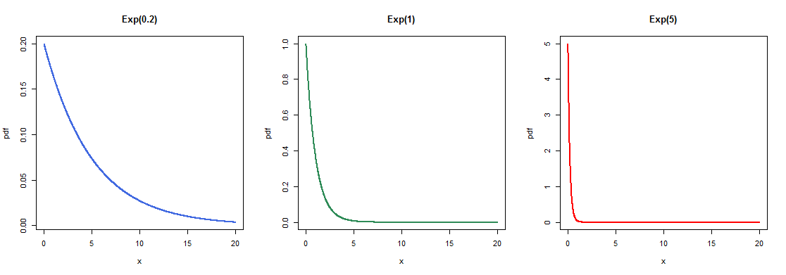
What does an Exponential distribution look like?
Below are some examples of what the pdf for various exponential distributions look like.

|center
Worked Example 2
Worked Example

The time in minutes, $X$, between the arrival of successive customers at a post office is exponentially distributed with pdf $f(x) = 0.2 e^{-0.2x}$.
(A) What is the expected time between arrivals?
(B) A customer walks into the post office at $12.30$p.m. What is the probability the next customer arrives:
(i) on or before $12:32$p.m.?
(ii) after $12:35$p.m.?
Solution
(A) Here $\lambda = 0.2$ and so the mean time between arrivals is $\frac{1}{0.2} = 5$ minutes.
(B) (i) If the next customer arrives on or before $12:32$p.m., it means that the time between their arrival and the previous arrival is at most $2$ minutes. So, we require $\mathrm{P}(X \leq 2)$.
Using the formula above we have:
\begin{align} \mathrm{P}(X \leq 2) &= 1 - e^{-0.2 \times 2}\\ &= 1 - 0.67032\\ &= 0.330 \text{ (to 3 d.p.)}\\ \end{align}
(ii) If the next customer arrives after $12:35$ p.m. then the time between the two customers is more than $5$ minutes. We now require $\mathrm{P}(X>5)$. To calculate $\mathrm{P}(X>x)$. This is equivalent to $1 - \mathrm{P}(X \leq x)$ and so:
\begin{align} \mathrm{P}(X > 5) &= 1 - \mathrm{P}(X \leq 5)\\ &= 1 - (1 - e^{-0.2 \times 5})\\ &= e^{-1}\\ &= 0.368 \text{ (to 3 d.p.)}.\\ \end{align}.
Poisson Processes
The Exponential distribution is often used as a model for the times between events. We have looked at events occurring randomly in time in association with the Poisson distribution. The Poisson distribution gives the probabilities for the number of events taking place in the given time period whereas the exponential distribution gives the probabilities for times between the events. Both of these concern events occurring randomly in time at a constant average rate, $\lambda$. This is known as a Poisson process.
For example, consider a series of randomly occurring events, such as customers entering a bank. The times of arrivals might look like this:
 .
.
There are two ways we can view the data.
- The number of arrivals in each minute ($1, 1, 0, 3, 1$).
- The times between successive arrivals.
For the Poisson process we have,
- the number of arrivals follows a Poisson distribution with parameter $\lambda$, and
- the time between successive calls has an exponential distribution with parameter $\lambda$.
Other Continuous Probability Distributions
There are other important continuous probability distributions which you will meet in practical business problems and decision making. In particular, you will meet the Student's t-distribution or t distribution and the Chi-squared ($\chi^2$) distribution. The t-distribution is used when testing a hypothesis about a mean or a difference between two means. The Chi-square distribution is used when analysing categorical data.
Test Yourself
Click on the following links to practise Numbas tests on the distributions on this page:
Test yourself: Numbas test on calculating probabilities from a normal distribution
Test yourself: Numbas test on the exponential distribution and uniform distribution