Numeracy, Maths and Statistics - Academic Skills Kit

Regression (Psychology)

ContentsToggle Main Menu 1 What is Regression? 2 Correlation Coefficient2.1 Important Note 3 Worked Example 4 Regression Equations 5 Reporting the Results 6 Worked Example 7 Test Yourself 8 See Also

What is Regression?

|250px

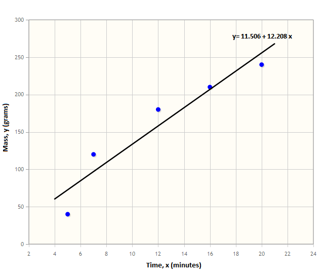
Regression methods find the line of best fit for a plot of two variables. To describe the regression line you need to calculate the $y$ intercept and the gradient of the line. Once you have this information you can estimate the most likely $Y$ value for a given $X$ value. You then use the standard error to calculate the probable spread of the estimates, this informs you of how your estimates may vary.

An example of regression in psychology content is large organisations comparing past employee psychometric test scores to those of new applicants. They can then make predictions for how successful they will be (e.g. a high test score may indicate a faster processing speed and therefore higher productivity rates etc.).

Correlation Coefficient

The correlation coefficient $(r)$ is a value between $-1$ and $+1$ and is a measure of how much $y$ varies due to $x$. When $r = 0$ this means there is no relationship. When $r = \pm 1$ this is a perfect relationship (the points lie exactly on a straight line). (For more information on this see correlation). The other values show the different levels of spread about the line of best fit.

If $r$ is positive then this equates to the regression line having a positive gradient (i.e. positive changes in $x$ result in positive changes in $y$), and if $r$ is negative then is has a negative gradient (i.e. a positive change in $x$ results in a negative change in $y$).

Note: This correlation coefficient is only valid if the relationship between the two variables is linear (i.e. not curved). To check for this, examine your plot and also check for outliers that may skew results.

The formula for calculating the correlation coefficient ($r$) is

\[r = \frac{\sum(x_i-\bar x)(y_i-\bar y)}{\sqrt{\sum(x_i-\bar x)^2\sum(y_i-\bar y)^2} }.\]

and more information can be found here although usually SPSS will calculate these values for you.

Important Note

The examples covered on this page are purely hypothetical and any results or data are not from any real studies nor cases. The purpose of them is to demonstrate how to use the various statistical methods covered in this section.

Worked Example

Worked Example - Correlation Coefficient

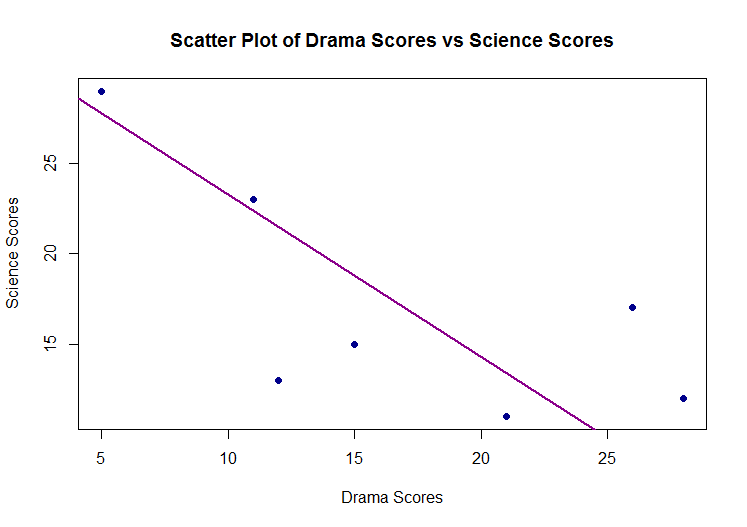
Below is a table and graph of science scores and drama scores from a primary school class. Some summary statistics have also been calculated too.

Calculate the correlation coefficient for this data.

$X$ - Drama Mark	$Y$ - Science Mark	$X^2$	$Y^2$	$XY$
$21$	$11$	$441$	$121$	$231$
$5$	$29$	$25$	$841$	$145$
$15$	$15$	$225$	$225$	$225$
$11$	$23$	$121$	$429$	$253$
$26$	$17$	$676$	$289$	$442$
$28$	$12$	$784$	$144$	$336$
$12$	$13$	$144$	$169$	$156$
$\sum X = 118$	$\sum Y = 120$	$\sum X^2 = 2416$	$\sum Y^2 = 2318$	$\sum XY = 1788$

|This is a scatter plot of the data with the line of best fit inputted

Solution

The values that we need for the formula have already been calculated for us, so we now need to input these into the above formula for the correlation coefficient, where our sample size $N = 7$

\[r = \dfrac{1788 - \dfrac{118 \times 120}{7}~}{\sqrt{\bigg(2416 - \dfrac{118^2}{7}\bigg)\bigg(2318 - \dfrac{120^2}{7}\bigg)}~} = - 0.704 \mathrm{\;(to\; 3d.p)}\]

So we have a negative correlation coefficient, which means that there is a substantial negative relationship between dramatic and scientific ability. This essentially equates to good scientists perform poorer in drama for this particular group of schoolchildren.

Regression Equations

This is another method of describing the relationship between two variables. It is different from the correlation coefficient as it allows those using it to make predictions from the data. A regression equation is one of the form:

\begin{equation} Y = a + bX \end{equation}

where: $Y$ is the predicted variable, $a$ is the $y$ intercept, $b$ is the regression coefficient and $X$ is the predictor variable.

You calculate $b$ and using the following formula found here although, usually you will use SPSS to calculate these values.

Reporting the Results

Firstly, note that interpretation of regression equations is only valid if the variables have a general linear relationship (i.e. do not lie on a curve).

A typical way to report findings could be: '' Due to the positive (or negative) correlation between the two variables, we were able to perform regression analysis on the data to find the slope $(b)$ and the $y$ intercept $(a)$. ''

Worked Example

Worked Example - Regression Equations

Using the information from the above worked example correlation coefficient. Calculate the regression equation, predict the science mark for a drama result of $19$ and then interpret your results.

Solution

The $\sum XY$, $\sum X$, $\sum Y $ and $\sum X^2$ values have already been calculated for us, so we can just substitute these values into the above equations for $a$ and $b$ to obtain the regression equation.

$b = \dfrac{1788 -\bigg(\dfrac{118 \times 120}{7}\bigg)}{2416 - \bigg(\dfrac{118^2}{7}\bigg) } = - 0.55 $ (2 d.p)

and

$a = \dfrac{120 - (b \times 118)}{7} = 26.42$ (2 d.p).

Thus our regression equation is: $ Y = 26.42 + (-0.55)X$.

Now predicting the science result if the student obtains a mark of $19$ in drama:

$Y = 26.42 + (-0.55)19 = 15.96 \approx 16$. So if a student obtained a mark of $19$ in their drama test then the prediction of their science score is approximately $16$.

Note: this is not exact, this is just our best guess at the outcome.

Due to the fact that the variables science scores and drama scores are negatively correlated, we can perform regression analysis to predict the science mark from knowing the drama mark. The slope of the regression of drama scores on science scores $b$ is $- 0.55$ and the $y$ intercept $a$ is $26.42.$

We can also perform this test in SPSS. To see how, watch the video tutorial below. As you can see, we get the same results as when we performed the test by hand.

Test Yourself

Try our Numbas test on regression.