Tests on Frequencies (Psychology)
Chi - Squared Tests
For quantitative data (numerical measurements), we use t-tests but they cannot be used for qualitative data (non numerical). For qualitative data, we use Chi-Squared Tests $(\chi^2$ tests$)$. Chi-Squared tests provide an objective method of investigating the probabilities of individuals being in specific categories/groups. We use Chi-Squared tests when we are dealing with frequencies rather than scores.
There are rules to follow when using a Chi-Squared test, listed below.
- No category has a mean of less than $5$.
- The categories should be as natural as possible.
- Keep to the raw data.
- Avoid categories that vastly exceed others.
Important Note
The examples covered on this page do not necessarily have the best experimental designs. They are also purely hypothetical and any results or data are not from any real studies nor experiments. The purpose of them is to demonstrate how to use the various hypothesis tests covered in this section.
The Method
- First, we form our hypotheses. Regardless of what the categorical variables are, if you are testing to see whether they are independent or not independent (associated) the hypotheses are:
\begin{align} H_0&: \text{There is }\textbf{no association}\text{ between the categorical variables versus}\\ H_1&: \text{There is }\textbf{an association}\text{ between the categorical variables.}\\ \end{align}
- After collecting the data, we calculate the test statistic.
\begin{equation} \chi^2 = \sum {\frac{(O-E)^2}{E}} \end{equation}
where:
\begin{align} O &= \text{Observed frequencies}\\ E &= \text{Expected frequencies}\\ \sum{} &=\text{Sum Of}\\ \end{align}
- We can get our expected frequencies by using the following formula:
\begin{equation} E = \; \dfrac{\text{row total} \times \text{column total}}{\text{overall sample size}} \end{equation}
for each cell in the contingency table.
- Once we have the test statistic, we can find a $p$-value/critical value. The appropriate degrees of freedom to use is given by:
\begin{equation} \nu = (\text{number of rows }- 1) \times (\text{number of columns} - 1) \end{equation}
- Finally, we form a conclusion. If the test statistics is greater than the critical value, we reject $H_0$ in favour of $H_1$. In other words, there is sufficient evidence to suggest that the two categorical variables are associated, or are not independent. Otherwise, we accept $H_0$.
See the worked example below.
One Sample Chi-Squared Tests
Sometimes in research we know the distribution in the population. It is possible to carry out a one sample Chi-Squared test if we know the population distribution of frequencies. Usually the population frequencies are known as relative frequencies or can be known in the form of percentages or proportions.
The Method
To carry out the test by hand, use the following steps.
- Firstly, we need to identify the null and alternative hypotheses $H_0$ and $H_1$.
- After collecting data, we calculate the expected frequencies based on our population distribution.
- We calculate the Chi-Square statistic/value:
\begin{equation} \chi^2 = \sum {\frac{(O-E)^2}{E}} \end{equation}
where:
\begin{align} O &= \text{Observed frequency}\\ E &= \text{Expected frequency}\\ \sum{} &=\text{ Sum Of}\\ \end{align}
- We then compare this statistic to a $\chi^2$ table on the appropriate degrees of freedom...
\begin{equation} \nu = (\text{number of categories}) - 1. \end{equation}
- Finally we make our conclusion. If the Chi-Squared value does not exceed the critical value (e.g. $p = 0.05$) then the null hypothesis will be accepted i.e. the data does follow the hypothetical pattern/population distribution. If it does exceed the critical value, the null hypothesis must be rejected.
See the worked example below.
Worked Examples
Worked Example - Chi-Squared Test
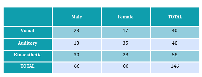
A psychologist wishes to test if preference of method of learning differs with gender. He asks a group of $146$ individuals their preferred method of learning. Below is a table of the results.
Perform a test to see if a relationship exists.

|center
Solution
Our hypotheses are: \begin{align} H_0:& \text{There is no relationship between preference of method of learning and gender.}\\ H_1:& \text{There is a relationship between preference of method of learning and gender.}\\ \end{align}
We need to calculate the expected frequencies before we can calculate the test statistic.
\begin{align} E_1 &= \; \dfrac{\text{row total for 'Visual'} \times \text{column total for 'Male'}}{\text{total number of participants}}\\ &= \dfrac{40 \times 66}{146}\\ &= 18.0822 \text{ (4 d.p.)}.\\ &\\ E_2 &= \; \dfrac{\text{row total for 'Visual'} \times \text{column total for 'Female'}}{\text{total number of participants}}\\ &= \dfrac{40 \times 80}{146}\\ &= 21.9178 \text{ (4 d.p.)}.\\ &\\ E_3 &= \; \dfrac{\text{row total for 'Auditory'} \times \text{column total for 'Male'}}{\text{total number of employees}}\\ &= \dfrac{48 \times 66}{146}\\ &= 21.6986 \text{ (4 d.p.)}.\\ &\\ E_4 &= \; \dfrac{\text{row total for 'Auditory'} \times \text{column total for 'Femalel'}}{\text{total number of particpants}}\\ &= \dfrac{48 \times 80}{146}\\ &= 26.3014 \text{ (4 d.p.)}.\\ &\\ E_5 &= \; \dfrac{\text{row total for 'Kinaesthetic'} \times \text{column total for 'Male'}}{\text{total number of employees}}\\ &= \dfrac{58 \times 66}{146}\\ &= 26.2192 \text{ (4 d.p.)}.\\ &\\ E_6 &= \; \dfrac{\text{row total for 'Kinaesthetic'} \times \text{column total for 'Female'}}{\text{total number of particpants}}\\ &= \dfrac{58 \times 80}{146}\\ &= 31.7808 \text{ (4 d.p.)}.\\ \end{align}
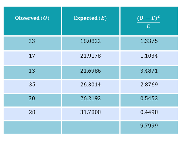
For convenience, we shall arrange the data into a new table to calculate the test statistic.

| center
Thus our test statistic is $\chi^2 = 9.8$ (3 d.p.).
We need to compare this to critical values on $\nu = (3 - 1) \times (2 -1) = 2$ degrees of freedom.

|center
Since $9.8 > 9.210$ (the critical value at the $1\%$ level) we can conclude there is very significant evidence that there is a relationship between preference of method of learning and gender for this particular group of participants. We accept $H_1$.
A concise way of writing up the results is as follows: 'There was a significant gender difference in preferred method of learning $(\chi^2 = 9.7999, \text{df} = 2, p <0.01)$
Worked Example - One-Sample Chi-Squared Test

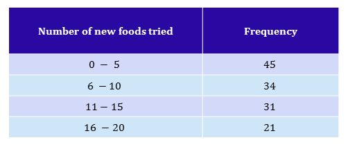
A psychologist is observing eating behaviour in $131$ children aged $3$ years old from Newcastle. He presents each child $20$ new foods which they have never eaten before. He then records the number of foods they actually try. The results are shown in the table below.
Previous research with thousands of children from across the country has shown that we expect $40\%$ of young children to try $0$ to $5$ new foods, $30\%$ to try $6$ to $10$ new foods, $20\%$ to try $11$ to $15$ new foods and $10\%$ to try $16$ to $20$ new foods.
Perform a test to see if the children from Newcastle follow the same distribution that the research on British children has found.

|center
Solution
Our hypotheses are: \begin{align} H_0&: \text{The children from Newcastle follow the same distribution found by the research.}\\ H_1&: \text{The children from Newcastle do not follow the same distribution found by the research.}\\ \end{align}
Firstly, we need to calculate the expected frequencies. We do this by multiplying the total number of children in the study by the expected proportions (from the national research).
\begin{align} E_1&= 40\% \times 131\\ &= 52.4\\ &\\ E_2&=30\% \times 131\\ &= 39.3\\ &\\ E_3&= 20\% \times 131\\ &=26.2\\ &\\ E_4&=10\% \times 131\\ &=13.1\\ \end{align}
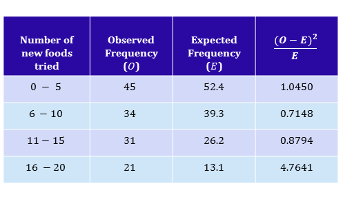
We can now input the expected frequencies into a table and calculate our test statistic.

|center
Our $\chi^2$ statistic is $1.0450 + 0.7148 + 0.8794 + 4.7641 = 7.4033$.
We then need to compare this to critical values on $\nu = 4 - 1 = 3$ degrees of freedom.

|center
Since $7.4033 < 7.815$ we do not have a significant value at the $5\%$ level. Therefore, we have no evidence to suggest that the children from Newcastle follow the same distribution as British children. We cannot reject $H_0$.
In a report we would write:
'It has been found that the children from Newcastle follow the same distribution as British children, when trying new foods. $(\chi^2 = 7.4033, \text{df} = 3, p > 0.05, \text{ns}).$'